XRFWin controls an x-ray spectrometer to acquire x-ray intensity as a function of energy or wavelength and will determine the composition, thickness or multi-layer thickness of a specimen using qualitative and quantitative analysis.
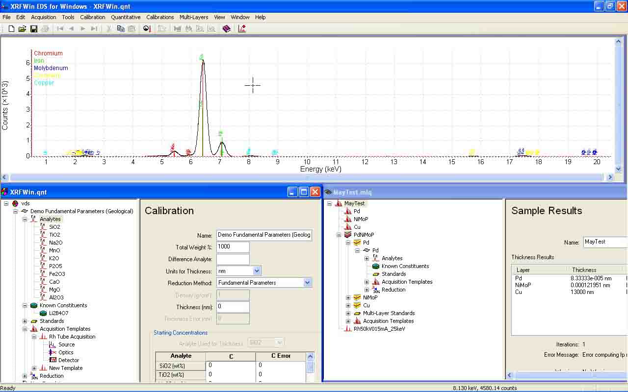
XRFWin is a comprehensive software package for performing qualitative and quantitative analysis using X-ray Florescence Spectroscopy. Qualitative analysis includes identifying the elements in a sample while quantitative analysis involves determining how much of each element is in the sample. Through a variety of data reduction methods, including the fundamental parameters method, corrections for matrix effects are made. The software also allows for the computation of layer thickness in a system of 1 or more layers.
Spectrometer drivers and an instrument abstraction layer means virtually any instrument can be directly controlled from within the software.
The software comes in two flavors; XRFWin WDS for wavelength-dispersive spectrometers, and XRFWin EDS for energy-dispersive spectrometers. For details regarding XRFWin WDS, please contact Omni Scientific Instruments, Inc.
The following refers to XRFWin EDS;
XRFWin runs on all Win32 operating systems including Windows 7, 8 and 10. The software is modular, each module adding capability. The basic package includes the ability to display and manipulate EDS spectra, and the spectrometer interface. The Qualitative Module adds the ability to identify elements in the spectra. The Quantitative Module adds the ability to determine the composition of bulk and thin samples and the thickness of a thin film. The Multi-Layer Module allows the determination of composition and layer thicknesses in a multi-layer sample.
Basic Package and Spectrometer Interface
- Interface with the spectrometer through an instrument abstraction layer. The abstract spectrometer is broken down into the Source, MCA with Detector Electronics, Enclosure and Sample Changer.
- Acquisition Templates allow rapid execution of repeated spectrometer configurations
- Simplified energy calibration
- Tools include ability to browse a database of the elements and explore overlapping characteristic lines
- Overlay known element lines on EDS spectra
Qualitative Analysis
- Identify atomic species in a sample from their characteristic lines
- Rich set of fitting and graphic tools to manipulate and analyze results.
- Results can be saved, printed or copied to the Windows clipboard
- Includes full database of the elements with interaction cross-sections and shell and characteristic line properties
- Includes a variety of tools for performing qualitative analysis
- Grid of atomic lines superimposed on spectrum
- Layover of atomic characteristic lines on spectrum
- Identification of peaks marked in graph
- Identification of elements from peak patterns in complete spectrum
- Identification of source Compton peaks
- Identification of detector escape peaks
- Peak profile fitting
Quantitative Analysis
- Determine element and compound concentrations from characteristic line intensity
- Determine thickness of single layer by volume integration
- Each analyzed element of calibration is termed an ‘analyte’ and may be associated with one or more other elements as a compound
- Calibrations may include known constituents such as in a flux preparation
- Calibrations may include one or more reference standards of known composition
- EDS Spectra extract line intensities by fitted peak profiles
- EDS Spectra account for overlap by simultaneously fitting overlapping peak profiles
- Determine x-ray penetration depth for a given calibration
- True fundamental parameters algorithm for data reduction
- Thickness measurements
- Composition measurements of thin film and bulk samples
- Includes primary absorption and secondary enhancement
- Includes effect of Coster-Kronig transitions
- Source x-ray spectrum can be line source or continuum with lines
- Tool for generating source x-ray tube spectrum
- Source spectrum can be measured or explicitly defined
- Option to use nearest standard or calibration curve
- Can interpolate calibration for missing standards
- Support for traditional empirical methods of data reduction
- Lachance and Traill
- Claisse and Quintin
- Rasberry and Heinrich
- Trace analysis by ratios
- Polynomial fit to standards
Multi-Layer Quantitative Analysis
- Determine concentration and/or layer thickness of one or more layers in a multi-layer system
- Each layer thickness determined by integrated volume or attenuation of an underlying layer characteristic line
- One or more layers may be of known thickness and concentration
- All multi-layer calculations utilize the fundamental parameters method
To understand x-ray fluorescence, an understanding of atomic structure is required. As much of the nomenclature of XRF spectroscopy has its roots in the history of the theory of atomic structure, an understanding of the historical development is helpful. The development of atomic structural theory can be broken down into three basic steps; Classical Atomic Theories, Old Quantum Theories and Modern Quantum Theories.
The production of characteristic x-rays in a sample is directly related to atomic transitions in the material.
Finally, the correlation of measured characteristic x-ray intensity with atomic concentration in a sample requires correction for the interaction of the x-rays with the sample medium - the so-called matrix affects
The following topics explore these ideas in more detail;
By 1910 it was clear from experiment that atoms contained negatively charged electrons, and that the number of electrons in an atom was roughly A/2 where A was its chemical atomic weight. Since atoms are usually neutral, there must have been an equal amount of positive charge within the atom. Since electrons were known to have a very small mass compared with the mass of the atom, the mass of the atom must have been associated with the positive charge.
The model of J. J. Thomson described the atom as having the electrons embedded in a sphere of positive charge. This model was qualitatively successful in that electromagnetic emission from the atom could be explained in terms of classical harmonic oscillation of the electrons of the atom. Evidence of agreement between predicted and observed emission spectra was not as convincing, however. Emission spectra were found to occur at discrete frequencies characteristic of the atom. Further, scattering of a particles (doubly ionized helium) indicated that the positive charge was concentrated in a very small volume 'nucleus' at the center of the atom.
Figure 1.2. Thomson's plum-pudding model of the atom showing scattering of an a particle.
Rutherford's model [1] of the hydrogen atom in 1911 had one electron orbiting a small heavy proton nucleus, attracted to the nucleus by a Coulomb interaction. This model appeared to agree with the physical structure of the atom, but the model implied that the hydrogen atom would be inherently unstable and there were still problems predicting the electromagnetic emission spectra of the atom. The electron could not have been stationary as it would simply be Coulomb attracted into the nucleus of the atom, resulting in an atomic diameter four orders of magnitude smaller than observed. An electron in a curved orbit is accelerated so must radiate electromagnetic energy. As energy is radiated, the radius of the electron orbit should decrease until the electron collapses into the nucleus. The Rutherford model predicted a typical lifetime of a hydrogen electron to be on the order of 10-10 seconds [2] and the radiated energy should have been continuous in energy.
Figure 1.3. Visible portion of the hydrogen spectrum. After Finkelnburg.
Atoms placed in an excited state, such as by passing electric current through a gas, were found to emit electromagnetic radiation concentrated at discrete frequencies. By passing the light emitted from an excited gas and then diffracting the light through a prism, this characteristic electromagnetic radiation appeared as lines on photographic plates. Similarly, atoms were found to absorb incident electromagnetic radiation at the same characteristic frequencies. The spectra of emitted radiation were found to be quite complicated for some atoms, but quite regular for the hydrogen atom. Attempts were made to identify series of progressively spaced lines in all elements, and empirical equations were derived to describe these series.
The discreteness of atomic electron energy levels was directly demonstrated in 1914 by the Frank-Hertz experiment. Passing electrons through a gas of a given atom to a grid at a given acceleration potential and then collecting the electrons at an anode at a lesser potential, drops in current were found when the acceleration voltage was increased beyond critical values. These drops in current corresponded to points where the electrons were accelerated to sufficient energy to excite electrons of the atom, losing energy in inelastic collisions. The electron energies remaining after the collision were then insufficient to overcome the reverse anode potential.
Clearly a model of the atom was needed that would at least predict the characteristic electromagnetic emission and absorption spectra observed in nature.
A black body is a material that absorbs perfectly at all wavelengths. The intensity of electromagnetic radiation emitted from a black body at some temperature is found to increase with frequency to some maximum (nm) and then decrease to zero at some greater frequency. The peak and maximum frequency of the envelope of emitted radiation is found to increase with temperature as shown in Figure 1.4. In the classical treatment, the black body radiator is described as a sea of electrons moving as harmonic oscillators in the walls of the object. This model predicted the intensity of the emitted radiation should increase quadratically with frequency. This agreed with experiment at low frequencies, but failed at higher frequencies.
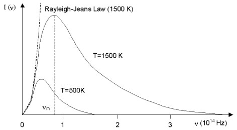
Figure 1.4. Black body radiator spectra distribution at 500K and 1500K. Dashed line at left shows the Rayleigh-Jeans Law of classical physics.
In 1900, Max Planck solved the problem of the black body radiator [3] by imposing conditions of quantization on the energies of the electron harmonic oscillators. Taking adjacent energy levels to be separated (ΔE) by an amount proportional to frequency (ν), he proposed:
\[ \Delta E = h \nu \: \: (1)\]
The constant h later came to be known as Planck's constant, and now has the accepted value 6.626x10⁻³⁴ J-sec.
An explanation for the spectral discreteness and stability of the hydrogen atom was provided by Bohr in 1913 [4]. In solving for the orbital motion of the electron in an orbit of radius r, Bohr imposed the condition that the angular momentum (l) of the electron must equal some integral multiple of h:
\[ pr = l = n \hbar = \frac{nh}{2 \pi} (n=1,2,3,4,...) \: \: (2)\]
where p is the linear momentum of the electron. He also postulated that electromagnetic radiation is emitted when an electron discontinuously changes its motion from one energy level to another, the frequency of the emitted radiation being as predicted by equation (1). As the difference in energies is equal to the energy of the emitted photon, the above relation is the same as Einstein's postulate that the energy of a photon is equal to its frequency times Planck's constant. On the basis of observation, Bohr also postulated that the feature of classical theory that predicted the emission of electromagnetic radiation by the orbiting electron was not valid for an atomic electron. With his restriction on the orbital angular momentum of the electron and suspension of an aspect of classical electromagnetic theory, the stability and energy levels of the hydrogen atom electrons were accurately predicted. This represented the first quantized model of the atom. The electron energy levels 'n' of hydrogen are shown in Figure 1.5. Electromagnetic emission corresponds to transitions of electrons between electron energy levels as shown.
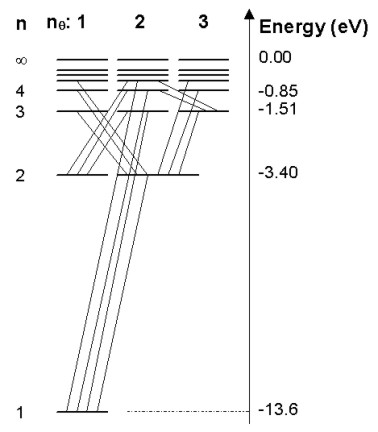
Figure 1.5. Electron energy levels of the hydrogen atom. Also shown are observed transitions between states resulting in emitted electromagnetic radiation. The 'n' quantum numbers represent orbitals predicted by Bohr's model while the 'l' quantum numbers indicate additional energy levels explained by Sommerfeld's model.
In nature, the energy levels of hydrogen predicted by the Bohr model are actually split into separate closely spaced energy levels. This 'fine structure' is seen in the energy levels of all atoms, but the Bohr model did not directly predict this. In 1916, Wilson and Sommerfeld proposed a quantum condition for physical systems that are periodic functions of time, called the Wilson-Sommerfeld rule. Planck's quantization of energy levels of the harmonic oscillator in the black body radiator and the quantization of angular momentum in the Bohr model were shown to be special cases of the Wilson-Sommerfeld rule.
Bohr's model described the orbit of the electron as circular. The Sommerfeld model [5] described the orbit of the electron as a generic ellipse. Using the Wilson-Sommerfeld rule, describing the electron orbit in polar co-ordinates lead to two integer quantum numbers n and nq, and therefore to sets of allowed elliptical orbits with each Bohr circular orbit.
\[ n_{\theta} = 1,2,3,...,n \: \: (3)\]
The set of spherical orbits associated with each circular orbit had the same total energy as the Bohr orbit unless account was made of relativity. In elliptical orbits, electrons pass closer to the nucleus than in circular orbits. Accordingly, electrons would travel faster as they approached the nucleus. By applying special relativity to the set of allowed elliptical orbits, Sommerfeld obtained the same fine structure of energy levels observed in hydrogen.
As indicated in Figure 1.5, not all transitions between energy levels resulting in the emission of a photon take place. The old quantum theory of atoms does not explain this. Though selection rules for transitions were established and the Correspondence Principle, described by Bohr in 1923, ensured consistency between model predictions and transition selection rules in the quantum and classical limits, the old quantum theory of the atom was an ad-hoc mixture of classical and quantum principles. The classical limit was defined as the point where quantum numbers describing the state of a system get very large.
The angular momentum condition of the Bohr atom was invented for the case of the hydrogen atom, and the model only worked reasonably well for one-electron atoms. The alkali elements (Li, Na, K, Rb, Cs) are similar to a one-electron atom, so limited success was found with these elements. In addition, the model says nothing about the rates at which transitions will occur. Finally, the Wilson-Sommerfeld rule limits the old quantum theory to periodic systems. There are many significant physical systems that are not periodic.
In 1924, de Broglie's doctoral thesis suggested the wave-particle duality of radiation (light waves and photons) was equally applicable to matter (electrons, etc.). As with radiation, the energy E of a particle is related to the frequency ν of the wave associated with its motion and the momentum p is related to the wavelength λ of the wave:
\[ E = h \nu \]
\[ p = h/ \lambda \: \: (4) \]
Substituting the second part of equation (4) into equation (2) results in:
\[ 2 \pi r = n \lambda \: \: (5) \]
As 2πr is the circumference of the orbit, the Bohr condition can be seen to be the same as requiring a standing wave around the atom. This new interpretation of matter led to the Schrödinger equation, quantum mechanics, and the modern quantum theory.
While the Bohr model has been replaced by quantum mechanics, its simplicity has ensured it is still a useful tool in the description of atomic physics. The persistence of such Bohr model concepts as 'orbital' in quantum physics is tribute to this.
As primary radiation penetrates into a specimen, it is absorbed. Once a fluoresced x-ray is emitted from an atom, it is also absorbed as it travels out of the sample toward the detection system. Further, fluoresced x-rays may act to enhance the intensity of fluoresced lower-energy x-rays. The absorption of primary radiation and absorption and enhancement of fluoresced characteristic lines is termed matrix effects.
The intensity of the emitted characteristic radiation should be related to the concentration of the associated element. However, to perform quantitative analysis the relation between element concentration and characteristic x-ray intensity needs to be established. The forms of the following equations are given to reflect the flow of this theory section. They do not necessarily follow the forms given by cited authors.
One of the early theoretical basis for using x-ray fluorescence to determine chemical composition of an unknown sample was proposed by von Hamos [7] in the 1940’s. He demonstrated that the emitted intensity of an element characteristic x-ray line in a binary system was proportional to the composition of that element in the specimen;
\[ R_i = C_i K_i \]
where Ri is the ratio between the measured x-ray intensity of element i in an unknown and the x-ray intensity measured for a pure specimen of element i. The constant Ki is a function of the composition of the specimen, the mass absorption coefficients of specimen constituents, and the measurement geometry. This equation represents a purely empirical method of determining element concentrations from measured counts or count rates.
Sherman Equation
Use of x-ray fluorescence to determine chemical composition of unknown specimens became more common in the following decade [8]. With this came the need to better understand x-ray absorption and enhancement. Sherman [9] derived a more specific equation for the fluoresced x-ray intensity from a multi-element specimen subjected to a monochromatic non-divergent incident radiation of energy E that only accounted for primary absorption;
\[ I_i = \frac{S \Omega}{4 \pi sin \psi_1 } \frac{C_i g_i \kappa(E_i,I_i) \mu_i(E) }{ \frac{\mu(E)}{sin \psi_1} + \frac{\mu(E_i)}{sin \psi_2}} \]
where
Ii Intensity of observed characteristic line of element i.
E Energy of incident radiation.
Ei Energy of the characteristic line of element i being measured.
S Irradiated surface area of specimen.
Ci Concentration of element i in the specimen.
gi Proportionality constant for characteristic line of element i.
θ1 Angle between the specimen surface and the incident x-rays.
θ2 Angle between the specimen surface and the detector.
Ω Solid angle subtended by the detector.
κ(Ei,Ii) Response of instrument at energy Ei of characteristic line energy of element i.
μi(E) Mass absorption coefficient of element i at incident energy E.
μ(E) Total absorption coefficient of specimen at incident energy E.
μ(Ei) Total absorption coefficient of specimen at characteristic line energy of element i.
Also note that;
\[ \mu(E) = \sum_j C_j \mu_j(E) \]
Sherman [10] later developed his theory to express the emitted x-ray intensity from a multi-element specimen subjected to a polychromatic radiation source. Sherman’s theory was then further refined by Shiraiwa and Fujino [11];
\[ I_i = \frac{J_i - 1}{J_i} \frac{s \Omega}{4 \pi sin \psi_1} \kappa(E_i,I_i) C_i p_i \omega_i \Bigg\{ \int_{E_{i edge}}^{E_{max}} I_o(E) \frac{\tau_i(E) dE}{ \frac{\mu(E)}{sin \psi_1} + \frac{\mu(E_i)}{sin \psi_2}} + \]
\[ ... C_j p_j \omega_j \sum_j \frac{J_j - 1}{2 J_j} \int_{E_{j edge}}^{E_{max}} \frac{\tau_i(E_j) \tau_j (E) }{ \frac{\mu(E)}{sin \psi_1} + \frac{\mu(E_i)}{sin \psi_2}}\]
\[ ... \left[ \frac{sin \psi_1}{\mu(E) } ln \left( 1 + \frac{\mu(E)}{\mu(E_j) sin \psi_1}\right) \frac{sin \psi_2}{\mu(E_i) } ln \left( 1 + \frac{\mu(E_i)}{\mu(E_j) sin \psi_2}\right) \right] dE \Bigg\} \]
where;
Ji Jump ratio of the photoelectric mass absorption coefficient at the absorption edge for the line of element i being measured.
ωi Fluorescent yield for the line of element i being measured.
Io(E) Intensity of incident radiation at energy E.
τi(E) Mass photoabsorption coefficient of element i at incident energy E.
τi(Ei) Mass photoabsorption coefficient of element i at energy Ei of characteristic line energy of element i.
pi Transition probability of observed line of element i.
Ei edge Energy of the absorption edge of the characteristic line of element i.
Emax Maximum energy of the incident radiation.
In general this equation is referred to as the Sherman equation. The sum over j is the sum over all characteristic lines of all elements strong enough to excite the observed line of element i. The first term in the above equation represents the primary absorption of the incident and characteristic line of element i in the specimen. The second term represents the secondary enhancement of the characteristic line of element i by all other characteristic lines fluoresced by the specimen. Though not included here, Shiraiwa and Fujino also gave an expression for the tertiary enhancement of the observed line of element i by all other characteristic lines in the sample.
The Sherman equation set the stage for modern x-ray fluorescence spectroscopy.
In the early days of modern x-ray fluorescence spectroscopy, the computing power required to determine the integrals of equation 5.4 was not readily available to spectroscopy laboratories. Thus efforts turned to empirical approximations to the above equations. Using Sherman’s first equation for an incident beam of monochromatic radiation (equation 5.2 above), Beattie and Brissey [12] showed that by taking the ratio between counts measured for element i in an unknown to the counts measured from a pure specimen of element i, a system of simultaneous equations was created;
\[ C_i/R_i = C_i + \sum_{i \neq j} C_j \left( \frac{\frac{\mu_i(E)}{sin \psi_1} + \frac{\mu_i(E_j)}{sin \psi_2}}{\frac{\mu_i(E)}{sin \psi_1} + \frac{\mu(E_i)}{sin \psi_2}} \right) = C_i + \sum_{i \neq j} A_{ij} C_j \]
\[ \sum_j C_j = 1\]
By measuring the intensity ratios Ri for a set of standards of known composition, this system of equations could be solved for each element in the substance to determine the constants Aij.
The appearance of Ci on both sides of equation 5.5 meant that the system of equations had to be solved numerically. Observing that concentration was roughly proportional to measured x-ray intensity, Lucas-Tooth and Pyne [13] rearranged the above equation to yield;
\[ C_i = a_i + b_i I_i \left( 1 + \sum_j k_{ij} I_j \right)\]
Once the parameters ai, bi, and kij had been determined using a set of standards, the concentration could be determined directly from this equation for each element in the specimen. Though limited in accuracy away from concentrations of the standards used to determine the coefficients, this method was highly attractive in the days before inexpensive laboratory computers.
Empirical Alpha Models
A problem with the formulation of Beatie and Brissey was that the system of equations had no constant terms and so was over-determined. In the mid sixties, LaChance and Traill [14] made the rather obvious observation that if equation 6 is substituted into equation 5, the over-determination of the system of equations was removed. This equation became the basis for the empirical alphas equations that followed;
\[ C_i = R_i \left( 1 + \sum_{i \neq j} \alpha_{ij} C_j \right) \]
Later attempts were made to find an empirical equation that more accurately accounted for the real relationship between measured x-ray intensity and specimen concentration. Claisse and Quintin [15] took the original Sherman equation (equation 5.2) and modeled for polychromatic incident radiation by taking the superposition of mass absorption coefficients at multiple energies. They obtained an equation of the form;
\[ C_i = R_i \left( 1 + \sum_{i \neq j} \alpha_{ij} C_j + \sum_{i \neq j,k} \alpha_{ijk} C_j C_k \right) \]
Though there is no direct theoretical support of this, it was generally found that the LaChance and Traill equation accounted for minor enhancement of x-ray intensities with negative alpha coefficients [17]. Rasberry and Heinrich [16] observed that strongly enhancing elements in binary mixtures yielded a concentration/intensity plot that did not follow the hyperbolic dependence of the LaChance and Traill equation. This led them to propose a modified form of the equation where a new term was to be used in place of the LaChance and Traill alpha coefficient for analytes causing significant secondary enhancement;
\[ C_i = R_i \left( 1 + \sum_{i \neq j} \alpha_{ij} C_j + \frac{\sum_{i \neq j} \beta_{ij} C_j}{1+C_i} \right) \]
By the middle of the 1970's, other forms of the alpha correction models had been proposed. Most notable are the equations of Tertian [18], [19] who, observing that alpha coefficients are more properly not constant with specimen composition, proposed forms of the LaChance and Traill, and Rasberry and Heinrich equations utilizing alpha coefficients that were linear functions of element concentration Ci. Later, Tertian also showed [20] that for a binary system, his modified form of the Rasberry and Heinrich equation reduced to the Claisse and Quintin equation.
Fundamental Parameters Method
Sherman’s equation (equation 5.4) expresses the intensity of a characteristic x-ray fluoresced from an element contained in a specimen of known composition. By determining the concentrations of elements required to produce the measured set of intensities the composition of a specimen can be determined. The direct use of Sherman’s equation is termed the fundamental parameters method. Instrument and measurement geometry effects are removed by measuring characteristic line intensities emanating from standards of known composition. Since this equation accounts for all absorption and enhancement, in theory only one standard is required for each element. It should be noted that the standard should also account for reflection from the surface of the specimen. As such, the surface texture of the standard should be similar to that of the unknown.
Equation 5.4 requires a knowledge of all elements contained in the specimen, the values of the total mass absorption and mass photoabsorption coefficients of each of these elements, and the step ratios of the mass photoabsorption coefficients at the absorption edges of the measured characteristic lines. A knowledge of the incident x-ray tube intensity distribution is also required. To account for secondary enhancement in the specimen, a knowledge of shell fluorescent yields and line transition probabilities are required.
Criss and Birks [21] were among the first to utilize the full fundamental parameters method. They were able to obtain uncertainties in concentrations for nickel and iron-base alloys between 0.1% and 1.7%. Aside from the requirement for significant computing power to evaluate the above integrals, the method is limited by the accuracy of the fundamental parameters themselves, and how well the tube spectrum is known. Determining a tube spectral distribution is no trivial matter. Due to the intensity of the primary radiation, direct measurement is not feasible. A common approach was to measure the reflected distribution from sugar, but then this involved properties of reflection. In the original Criss and Birks paper, the measured spectra of Gilfrich and Birks [22] were utilized. Later developments either continued to use the spectra of Gilfrich and Birks [23], allowed user-entered spectra which usually implied the use of the spectra of Gilfrich and Birks [24], [25], [26], or utilized Kramer’s Law to generate the spectrum [27].
The need for computing power sufficient to evaluate the above integral and the lack of good knowledge of the tube spectrum led a number of authors to the use of an effective incident wavelength in place of the actual tube spectral distribution [28], [29], [30], [31]. Comparisons between fundamental parameters software packages utilizing effective wavelength and tube spectral distributions have demonstrated the shortcomings of this approach [32].
The strength of the fundamental parameters method is that only one standard is required. Since the method predicts the degree of correction for a given composition, a single standard should be sufficient for all ranges of composition of an unknown specimen. Empirical alpha models of correction require significantly more standards, and these standards need to be of similar composition to the unknown being analyzed. Early developments of the fundamental parameters method noted that most of the fundamental parameters drop out for a pure substance. Taking the ratio between x-ray intensities measured from the unknown specimen to those measured from pure substances allowed the most direct use of the fundamental parameters method. As noted by Sherman himself, and later by Criss, Birks and Gilfrich [33], this tends to increase the reliance on the fundamental parameters that are known to be in error by as much as 10% [34]. The degree of correction (and so the error in correction) is reduced by using standards similar in composition to the unknown.
Fundamental Alphas
The strength of the fundamental parameters method is that it is theoretically exact, and requires relatively few standards. Aside from the need for accurate fundamental parameters and a knowledge of the x-ray tube spectrum, the fundamental parameters method is numerically intensive, and so could take a significant amount of time to compute the composition of a specimen on early laboratory mini-computers. To take advantage of the few number of standards required by the fundamental parameters method and the relatively small computing resource needed for the empirical alphas methods, the hybrid fundamental alphas method came into being [35], [36]. These methods use the fundamental parameters method on larger computing facilities to compute empirical coefficients that are later used in traditional empirical alphas equations on a smaller laboratory computer [37], [38].
There are different methods used to compute theoretical alpha coefficients. One approach involves computing synthetic standards using the fundamental parameters method, and then computing the empirical alphas using standard regression techniques [33], [39]. Another approach is to compute the empirical alpha coefficients directly from Sherman’s equation for binary systems [40], [41]. Rouseau [42] proposed a new empirical alphas equation that can be more directly related to Sherman’s equation;
\[ C_i = R_i \frac{1 + \sum_j C_j \alpha_{ij}}{1 + \sum_j C_j \rho_{ij}} \]
where ρij are another set of alpha coefficients.
As noted by LaChance [43], the fundamental parameters method and theoretical alphas of the fundamental alphas method rely on inherently different concepts. This means that the flexibility gained by the fundamental alphas approach implies a loss of the ability to define those coefficients explicitly from theory.
It is our opinion that with the increase in laboratory computing power available by the mid 1990’s, the need for compromise with the fundamental parameters method has vanished.
Other Approaches
Other methods of reducing measured counts to element concentrations arise under special circumstances. Particularly for geological samples containing heavy trace elements, the integral of the Sherman equation will sometimes reduce to a constant value for the heavy trace elements. This constant is a function of absorption in the sample, and through the observation that the ratio between mass absorption coefficients at a given energy is roughly independent of energy [44], the so-called Ratio method has evolved. To improve counting statistics, the Compton-scattered primary radiation peak, also dependent on total sample mass-absorption is often used.
Semi-Quantitative Analysis
A throw-back to the early days of XRF spectroscopy is semi-quantitative analysis. This method of matrix correction involved simply computing the concentration of an element from the product of the unknown to standard intensity ratio with the concentration of the element in the standard. More sophisticated so-called quantitative analysis methods utilized polynomials and peak counts corrected for background. These approaches are both mathematically and theoretically simplistic, and with well-designed modern XRF software, are completely unnecessary. XRFWIN includes the Polynomial Fit to Standards matrix correction method for legacy support, but most analysis such as quantitative analysis of a qualitative scan should utilize the fundamental parameters method.
The following is a list of references cited for x-ray fluorescence.
-
E. Rutherford, Phil. Mag. 21, 669, 1911.
-
A. Yariv, "Theory and Applications of Quantum Mechanics", John Wiley & Sons, Inc., 1982.
-
M. Planck, Ann. Phys. 4, 553, 1901.
-
N. Bohr, Phil. Mag. 26, 476, 1913.
-
A. Sommerfeld, Ann. Phys. (Leipzig) 51, 1, 1916.
-
W. Finkelnburg, "Structure of Matter", Springer-Verlag, Heidelburg, 1964.
-
von Hamos, L., Arkiv. Math. Astron. Fys. 31a, 25, 1945.
-
Gillam, E., Heal, H.T., British Journal of Applied Physics, Vol. 3, pg. 353-358, 1952.
-
Sherman, J., ASTM Special Tech. Publ. No. 157, 1954.
-
Sherman, J., Spectrochim. Acta. 7, 283, 1955.
-
Shiraiwa, T., Fujino, N., Japanese Journal of Applied Physics, Vol. 5, No. 10, pg. 886-899, October 1966.
-
Beattie, H.J., Brissey, R.M., Analytical Chemistry, Vol. 26, No. 6, pg. 980-983, June 1954.
-
Lucas-Tooth, J., Pyne, C., Advances in X-ray Analysis, Vol. 7, pg. 523-541, 1963.
-
LaChance, G.R., Traill, R.J., Canadian Spectroscopy, Vol. 11, pg. 43-48, March 1966.
-
Claisse, F., Quintin, M., Canadian Spectroscopy, Vol. Vol. 12, pg. 129-146, September 1967.
-
Rasberry, S.D., Heinrich, K.F.J., Analytical Chemistry, Vol. 46, No. 1, pg. 81-89, January 1974.
-
Traill, R.J., LaChance, G.R., Canadian Spectroscopy, Vol. 11, pg. 63-70, May 1966.
-
Tertian, R., X-ray Spectrometry, Vol. 2, pg. 95-109, 1973.
-
Tertian, R., X-ray Spectrometry, Vol. 3., pg. 102-108, 1974.
-
Tertian, R., Advances in X-ray Analysis, Vol. 19, pg. 85-111, 1976.
-
Criss, J.W., Birks, L.S., Analytical Chemistry, Vol. 40, No. 7, pg. 1080-1086, June 1968.
-
Gilfrich, J.V., Birks, L.S., Analytical Chemistry, Vol. 40, No. 7, pg. 1077-1080, June 1968.
-
Gould, R.W., Bates, S.R., X-ray Spectrometry, Vol. 1, pg. 29-35, 1972.
-
Laguitton, D., Mantler, M., Advances in X-ray Analysis, Vol. 20, pg. 515-528, 1977.
-
Huang, T.C., X-ray Spectrometry, Vol. 10, No. 1, pg. 28-30, 1981.
-
Mantler, M., Advances in X-ray Analysis, Vol. 27, pg. 433-440, 1984.
-
Pohn, C., Ebel, H., Advances in X-ray Analysis, Vol.. 35, pg.715-720, 1992.
-
Sparks, C.J., Advances in X-ray Analysis, Vol. 19, pg. 19-52, 1976.
-
Shen, R.B., Russ, J.C., X-ray Spectrometry, Vol. 6, No. 1, pg. 56-61, 1977.
-
Quinn, A.P., Advances in X-ray Analysis, Vol. 22, pg. 293-302, 1978.
-
Tertian, R., Vie le Sage, R., X-ray Spectrometry, Vol. 5, pg. 73-83, 1976.
-
Bilbrey, D.B., Bogart, G.R., Leyden, D.E., Harding, A.R., X-ray Spectrometry, Vol. 17, pg. 63-73, 1988.
-
Criss, J.W., Birks, L.S., Gilfrich, J.V., Analytical Chemistry, Vol. 50, No. 1, January 1978
-
Vrebos, B.A.R., Pella, P.A., X-ray Spectrometry, Vol. 17, pg. 3-12, 1988.
-
de Jongh, W.K., X-ray Spectrometry, Vol. 2, pg. 151-158, 1973.
-
Rousseau, R., Claisse, F., X-ray Spectrometry, Vol. 3, pg. 31-36, 1974.
-
Kalnicky, D.J., Advances in X-ray Analysis, Vol. 29, pg. 451-460, 1986.
-
Jenkins, R., Croke, J.F., Niemann, R.L., Westberg, R.G., Advances in X-ray Analysis, Vol. 18, pg. 372-381, 1975.
-
Criss, J.W., Advances in X-ray Analysis, Vol. 23, pg. 93-97, 1980.
-
Broll, N., Tertian, R., X-ray Spectrometry, Vol. 12, No. 1, pg. 30-37, 1983.
-
Tertian, R., X-ray Spectrometry, Vol. 17, pg. 89-98, 1988.
-
Rousseau, R.M., X-ray Spectrometry, Vol. 13, No. 3, pg. 115-125, 1984.
-
LaChance, G.R., Advances in X-ray Analysis, Vol. 31, pg. 471-478, 1988.
-
Hower, J., American Mineralogist, Vol. 44, 19-32, 1959.
The following details the price structure for a license to use XRFWin EDS. All prices are in US dollars:
|
Item |
Price |
|
XRFWin EDS Basic Package (Includes spectrometer interface) |
Free |
|
Qualitative Analysis |
$499.00 |
|
Quantitative Analysis |
$2499.00 |
|
Multi-Layer Quantitative Analysis |
$1499.00 |
Contact TASI Technical Software for additional information
Export of INI format for multilayer could index the wrong acquisition template name
Attenuation of overlying layers could calculate crash calculation for sources with no continuum
Importing spectra from files might not assign import settings properly
Added AngstromeExcellence Import format
Modified XRFWin Import format to include count time and live time
Modified Execute automation functions so do not require count and live time
Possible disruption of source continuum integration if duplicates in source spectrum
Added reading of energy for imported spectra from acquisition template
Reorganised import text spectrum code
Added trap for zero angle condition
Normalized generated source continuum to 1e6
Enhanced Execute automation functions to support calibrations with multiple acquisition templates
Possible corruption adding new acquisition templates caused by double destruction
Memory leak if utilize non port-based devices
CAL was not loading acquisition template drift corrections when creating QNT (MAL was ok for MLQ)
Quick Drift correction was incorrectly deflating standard intensities for added standard when should have inflated them to theoretical 'original' instrument when re-acquiring standard
Added Rontec driver
Updated help for EDS import text file formatting
Added Execute COM members for analysis-only
Under certain circumstances a memory leak could occr when making a new run from Acquisition|AcquireSpectrum
Updated XIA Handel interface to 1.2.24
Added ability to fix peak energy while fitting profiles in quantitative analysis
QNTProfileFitSettings copy constructor not copying UseBck
Changed to new activation server
Thickness by polynomial added uncertainty to thickness due to counting stats and optionally uncertainty in coefficients
Use Background checkbox not being updated in Acquisition Templates Marked Peaks dialogue interface